Terzaghi Porous Media Mechanics Problem

This repository contains the codes used to generate the example presented in Lavigne et al., 2023 [1] (published as an open-source tutorial article in JMBBM journal). This article provides a precise and complete tutorial of the following.

This examples focus on uni-axial confined compression of a column sample as show below.

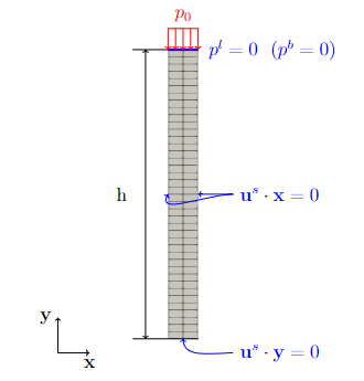
For such problem, the analytical Terzaghi solution is defined by:

\[\text{p(z,t)}=\frac{4p_0}{\pi}\sum_{k=1}^{+\infty}\frac{(-1)^{k-1}}{2k-1}\cos[(2k-1)\frac{\pi}{2}\frac{z}{h}]\exp[-(2k-1)^2\frac{\pi^2}{4}\frac{c_vt}{h^2}]\]

\[c_v = \frac{k^\varepsilon}{\mu^l(S+\frac{\beta^2}{M})}\]

\[M = \frac{3K^s(1-\nu)}{(1+\nu)}\]

\[S = \frac{\beta-\varepsilon^l_0}{K^s} + \frac{\varepsilon^l_0}{K^l}\]

Implementation

Libraries and python functions

Similarly to the other examples, the first step is to import the libraries.

import numpy
import time
import dolfinx
import ufl
import mpi4py
import basix
import petsc4py
# 
from dolfinx.fem.petsc import NonlinearProblem
from dolfinx.nls.petsc import NewtonSolver

We can then define the useful functions for the rest of the computation:

• Elasticity Law :

\[2\mu\mathbf{\epsilon}(\mathbf{u}^s)+\lambda \text{tr}(\mathbf{\epsilon}(\mathbf{u}^s))\mathbf{I_d},\]

• Terzaghi analytical solution in space,

• L2 error function in pressure :

\[E({p^l})~=~\frac{\sqrt{\int_\Omega (p^l-p^{ex})^2\mathrm{d} x}}{\sqrt{\int_\Omega (p^{ex})^2\mathrm{d} x}},\]

• Evaluation of a function for a physical point,

• Terzaghi solution in time for the top points.

def Hookean(u):
    """
    Compute the effective stress tensor
    Inputs: displacement vector
    Outputs: effective stress
    """
    return lambda_m * ufl.nabla_div(u) * ufl.Identity(len(u)) + 2*mu*ufl.sym(ufl.grad(u))
# 
def terzaghi_p(x):
    """
    Compute the Exact Terzaghi solution
    Inputs: coordinates
    Outputs: Fluid pressure 
    """
    kmax = 1e3
    p0,L = pinit, Height
    cv   = permeability.value/viscosity.value*(lambda_m.value+2*mu.value)
    pression = 0
    for k in range(1,int(kmax)):
        pression += p0*4/numpy.pi*(-1)**(k-1)/(2*k-1)*numpy.cos((2*k-1)*0.5*numpy.pi*(x[1]/L))*numpy.exp(-(2*k-1)**2*0.25*numpy.pi**2*cv*t/L**2)
    pl = pression
    return pl
# 
def L2_error_p(mesh,P1,__p):
    """
    Define the L2_error computation
    Inputs: Mesh, type of element, solution function
    Outputs: L2 error to the analytical solution
    """
    P1space = dolfinx.fem.functionspace(mesh, P1)
    p_theo  = dolfinx.fem.Function(P1space)
    p_theo.interpolate(terzaghi_p)
    L2_errorp, L2_normp = dolfinx.fem.form(ufl.inner(__p - p_theo, __p - p_theo) * dx), dolfinx.fem.form(ufl.inner(p_theo, p_theo) * dx)
    num_local = dolfinx.fem.assemble_scalar(L2_errorp)
    den_local = dolfinx.fem.assemble_scalar(L2_normp)

    num = mesh.comm.allreduce(num_local, op=mpi4py.MPI.SUM)
    den = mesh.comm.allreduce(den_local, op=mpi4py.MPI.SUM)
    return numpy.sqrt(num / den)
# 
def evaluate_point(mesh, function, contributing_cells, point, output_list, index):
    """
    Suitable Evaluations functions for Parallel computation
    Inputs: mesh, function to evaluate, contributing cells to the point, point, output list to store the value, index in the list
    Outputs: the evaluated function value is added at the index location in output list
    """
    from mpi4py            import MPI
    function_eval = None
    if len(contributing_cells) > 0:
        function_eval = function.eval(point, contributing_cells[:1])
    function_eval = mesh.comm.gather(function_eval, root=0)
    # Choose first pressure that is found from the different processors
    if mpi4py.MPI.COMM_WORLD.rank == 0:
        for element in function_eval:
            if element is not None:
                output_list[index]=element[0]
                break
    pass
# Terzaghi analytical solution
def terzaghi(p0,L,cv,y,t,kmax):
    """
    y as the position, t as the time we are looking to
    p0 the applied pressure
    L the sample's length
    cv the consolidation time
    """
    pression=0
    for k in range(1,kmax):
        pression += p0*4/numpy.pi*(-1)**(k-1)/(2*k-1)*numpy.cos((2*k-1)*0.5*numpy.pi*(y/L))*numpy.exp(-(2*k-1)**2*0.25*numpy.pi**2*cv*t/L**2)
    pl = pression
    return pl

Mesh creation and marking

The mesh is created within FEniCSx:

## Create the domain / mesh
Height = 1e-4 #[m]
Width  = 1e-5 #[m]
mesh   = dolfinx.mesh.create_rectangle(mpi4py.MPI.COMM_WORLD, numpy.array([[0,0],[Width, Height]]), [2,40], cell_type=dolfinx.mesh.CellType.triangle)

The boundaries are marked using (tag, locator) tuples:

# 1 = bottom, 2 = right, 3=top, 4=left
boundaries = [(1, lambda x: numpy.isclose(x[1], 0)),
              (2, lambda x: numpy.isclose(x[0], Width)),
              (3, lambda x: numpy.isclose(x[1], Height)),
              (4, lambda x: numpy.isclose(x[0], 0))]
# 
facet_indices, facet_markers = [], []
fdim = mesh.topology.dim - 1
for (marker, locator) in boundaries:
    facets = dolfinx.mesh.locate_entities_boundary(mesh, fdim, locator)
    facet_indices.append(facets)
    facet_markers.append(numpy.full_like(facets, marker))
# Concatenate and sort the arrays based on facet indices. Left facets marked with 1, right facets with two
facet_indices = numpy.hstack(facet_indices).astype(numpy.int32)
facet_markers = numpy.hstack(facet_markers).astype(numpy.int32)
sorted_facets = numpy.argsort(facet_indices)
facet_tag     = dolfinx.mesh.meshtags(mesh, fdim, facet_indices[sorted_facets], facet_markers[sorted_facets])
# 
# 
with dolfinx.io.XDMFFile(mpi4py.MPI.COMM_WORLD, "tags.xdmf", "w") as xdmf:
    xdmf.write_mesh(mesh)
    xdmf.write_meshtags(facet_tag,mesh.geometry)

Similarly the cells contributing to the physical points for evaluation are identified:

# Identify contributing cells to our points of interest for post processing
num_points = 11
# Physical points we want an evaluation in
y_check          = numpy.linspace(0,Height,num_points)
points_for_time  = numpy.array([[Width/2, 0., 0.], [Width/2, Height/2, 0.]])
points_for_space = numpy.zeros((num_points,3))
for ii in range(num_points):
    points_for_space[ii,0] = Width/2
    points_for_space[ii,1] = y_check[ii]
# Create the bounding box tree
tree             = dolfinx.geometry.bb_tree(mesh, mesh.geometry.dim)
points           = numpy.concatenate((points_for_time,points_for_space))
cell_candidates  = dolfinx.geometry.compute_collisions_points(tree, points)
colliding_cells  = dolfinx.geometry.compute_colliding_cells(mesh, cell_candidates, points)
cells_y_0        = colliding_cells.links(0)
cells_y_H_over_2 = colliding_cells.links(1)

Mechanical parameters and loading

The material, temporal and load parameters are defined:

## Time parametrization
t         = 0                # Start time
Tf        = 6.           # End time
num_steps = 1000             # Number of time steps
dt        = (Tf-t)/num_steps # Time step size
# Poromechanical parameters
E            = dolfinx.default_scalar_type(5000)
nu           = dolfinx.default_scalar_type(0.4)
lambda_m     = dolfinx.fem.Constant(mesh, dolfinx.default_scalar_type(E*nu/((1+nu)*(1-2*nu))))
mu           = dolfinx.fem.Constant(mesh, dolfinx.default_scalar_type(E/(2*(1+nu))))
rhos         = dolfinx.fem.Constant(mesh, dolfinx.default_scalar_type(1))
permeability = dolfinx.fem.Constant(mesh, dolfinx.default_scalar_type(1.8e-15)) 
viscosity    = dolfinx.fem.Constant(mesh, dolfinx.default_scalar_type(1e-2))  
rhol         = dolfinx.fem.Constant(mesh, dolfinx.default_scalar_type(1))
beta         = dolfinx.fem.Constant(mesh, dolfinx.default_scalar_type(1))
porosity     = dolfinx.fem.Constant(mesh, dolfinx.default_scalar_type(0.2))
Kf           = dolfinx.fem.Constant(mesh, dolfinx.default_scalar_type(2.2e9))
Ks           = dolfinx.fem.Constant(mesh, dolfinx.default_scalar_type(1e10))
S            = (porosity/Kf)+(1-porosity)/Ks
# 
## Mechanical loading 
pinit = 100 #[Pa]
T     = dolfinx.fem.Constant(mesh,dolfinx.default_scalar_type(-pinit))

Function Spaces, Functions and Operators

The mixed function space, (u,p) in (P2v,P1) for stability concerns, is computed. The solution and function at the previous time step are defined as well as the operators for the variationnal form:

# Finite Element 
P1   = basix.ufl.element("P", mesh.topology.cell_name(), degree=1)
# Vector Element
P2_v = basix.ufl.element("P", mesh.topology.cell_name(), degree=2, shape=(mesh.topology.dim,))
# 
MS   = dolfinx.fem.functionspace(mesh, basix.ufl.mixed_element([P2_v,P1]))
# 
#----------------------------------------------------------------------
# Functions
# Create the initial and solution functions of space
X0 = dolfinx.fem.Function(MS)
Xn = dolfinx.fem.Function(MS)
# Identify the unknowns from the function
u,p     = ufl.split(X0)
u_n,p_n = ufl.split(Xn)
# Set up the test functions
v,q     = ufl.TestFunctions(MS)
dX0     = ufl.TrialFunction(MS)
#----------------------------------------------------------------------
# Operators
# Create the surfacic element
metadata = {"quadrature_degree": 4}
dx       = ufl.Measure("dx", domain=mesh, metadata=metadata)
ds       = ufl.Measure("ds", domain=mesh, subdomain_data=facet_tag)
# compute the mesh normals to express t^imposed = T.normal
normal   = ufl.FacetNormal(mesh)

Boundary and Initial conditions

The boundary conditions in displacement and pressure are imposed:

# 1 = bottom: uy=0, 2 = right: ux=0, 3=top: pl=0 leakage, 4=left: ux=0
bcs    = []
fdim   = mesh.topology.dim - 1
# uy=0
facets = facet_tag.find(1)
dofs   = dolfinx.fem.locate_dofs_topological(MS.sub(0).sub(1), fdim, facets)
bcs.append(dolfinx.fem.dirichletbc(dolfinx.default_scalar_type(0), dofs, MS.sub(0).sub(1)))
# ux=0
facets = facet_tag.find(2)
dofs   = dolfinx.fem.locate_dofs_topological(MS.sub(0).sub(0), fdim, facets)
bcs.append(dolfinx.fem.dirichletbc(dolfinx.default_scalar_type(0), dofs, MS.sub(0).sub(0)))
# ux=0
facets = facet_tag.find(4)
dofs   = dolfinx.fem.locate_dofs_topological(MS.sub(0).sub(0), fdim, facets)
bcs.append(dolfinx.fem.dirichletbc(dolfinx.default_scalar_type(0), dofs, MS.sub(0).sub(0)))
# leakage p=0
facets = facet_tag.find(3)
dofs   = dolfinx.fem.locate_dofs_topological(MS.sub(1), fdim, facets)
bcs.append(dolfinx.fem.dirichletbc(dolfinx.default_scalar_type(0), dofs, MS.sub(1)))

The initial conditions are introduced as follows:

Un_, Un_to_MS = MS.sub(0).collapse()
Pn_, Pn_to_MS = MS.sub(1).collapse()

# For displacement
FUn_ = dolfinx.fem.Function(Un_)
FUn_.x.array[:] = 0.0  # set all DOFs to zero
FUn_.x.scatter_forward()

# For pressure
FPn_ = dolfinx.fem.Function(Pn_)
FPn_.x.array[:] = pinit  # set all DOFs to pinit
FPn_.x.scatter_forward()

Xn.x.array[Un_to_MS] = FUn_.x.array
Xn.x.array[Pn_to_MS] = FPn_.x.array
Xn.x.scatter_forward()

Variationnal form

The problem is extensively described in Lavigne et al., 2023. The variationnal form is the following:

\[\begin{split} \begin{split} \frac{S}{dt}\int_{\Omega} (p^l-p^l_n)q\text{d}\Omega+\frac{1}{dt}\int_{\Omega} \mathbf{\nabla}\cdot(\mathbf{u}^s-\mathbf{u}^s_n)q\text{d}\Omega \\ + \frac{k^\varepsilon}{\mu^l} \int_{\Omega} \mathbf{\nabla}p^l\mathbf{\nabla}q\text{d}\Omega = 0, \forall~ q\in~\text{L}_0^2(\Omega) \end{split} \end{split}\]

\[\begin{split} \begin{split} \int_{\Omega} \mathbf{t}^\text{eff}:\mathbf{\nabla}\mathbf{v}\text{d}\Omega-\int_{\Omega}\beta p^l\mathbf{\nabla}\cdot\mathbf{v}\text{d}\Omega - \int_{\Gamma_s} \mathbf{t}^\text{imposed} \cdot \mathbf{n} \cdot \mathbf{v} \text{d}\Gamma_s=0,\\ \forall~\mathbf{v}\in~[\text{H}^1(\Omega)]^2 \end{split} \end{split}\]

F       = (1/dt)*ufl.nabla_div(u-u_n)*q*dx + (permeability/viscosity)*ufl.dot(ufl.grad(p),ufl.grad(q))*dx  + ( S/dt )*(p-p_n)*q*dx
F      += ufl.inner(ufl.grad(v),Hookean(u))*dx - beta * p * ufl.nabla_div(v)*dx - T*ufl.inner(v,normal)*ds(3)

Problem Definition

The problem and solver settings are defined.

# Non linear problem definition
J       = ufl.derivative(F, X0, dX0)
Problem = NonlinearProblem(F, X0, bcs = bcs, J = J)
#
#---------------------------------------------------------------------- 
# set up the non-linear solver
solver  = NewtonSolver(mesh.comm, Problem)
# Absolute tolerance
solver.atol = 5e-10
# relative tolerance
solver.rtol = 1e-11
# Convergence criterion
solver.convergence_criterion = "incremental"
# 
# Maximum iterations
solver.max_it                = 15
# Solver Pre-requisites
ksp                                               = solver.krylov_solver
opts                                              = petsc4py.PETSc.Options()
option_prefix                                     = ksp.getOptionsPrefix()
opts[f"{option_prefix}ksp_type"]                  = "preonly"
opts[f"{option_prefix}pc_type"]                   = "lu"
opts[f"{option_prefix}pc_factor_mat_solver_type"] = "mumps"
ksp.setFromOptions()

Post-processing and Solving

Lists and export files are initialised for post processing

xdmf = dolfinx.io.XDMFFile(mesh.comm, "Result.xdmf", "w")
xdmf.write_mesh(mesh)
# Create output lists in time and space for the IF pressure
pressure_y_0 = numpy.zeros(num_steps+1, dtype=dolfinx.default_scalar_type)
pressure_y_Height_over_2 = numpy.zeros(num_steps+1, dtype=dolfinx.default_scalar_type)
pressure_space0 = numpy.zeros(num_points, dtype=dolfinx.default_scalar_type)
pressure_space1 = numpy.zeros(num_points, dtype=dolfinx.default_scalar_type)
pressure_space2 = numpy.zeros(num_points, dtype=dolfinx.default_scalar_type)
# initial conditions
pressure_y_0[0] = pinit
pressure_y_Height_over_2[0] = pinit

The solution is computed for each time step:

# time steps to evaluate the pressure in space:
n0, n1, n2 = 200,400,800
# 
t = 0
L2_p = numpy.zeros(num_steps, dtype=dolfinx.default_scalar_type)
for n in range(num_steps):
    t += dt
    try:
        num_its, converged = solver.solve(X0)
    except:
        if mpi4py.MPI.COMM_WORLD.rank == 0:
            print("*************") 
            print("Solver failed")
            print("*************") 
            break
    X0.x.scatter_forward()
    # Update Value
    Xn.x.array[:] = X0.x.array
    Xn.x.scatter_forward()
    __u, __p = X0.split()
    # 
    # Export the results
    __u.name = "Displacement"
    __p.name = "Pressure"
    # Export U to degree one for export
    # xdmf.write_function(__u,t)
    xdmf.write_function(__p,t)
    # 
    # Compute L2 norm for pressure
    error_L2p     = L2_error_p(mesh,P1,__p)
    L2_p[n] = error_L2p
    # 
    # Solve tracking
    if mpi4py.MPI.COMM_WORLD.rank == 0:
        print(f"Time step {n}/{num_steps}, Load {T.value}, L2-error p {error_L2p:.2e}") 
    # Evaluate the functions
    # in time
    evaluate_point(mesh, __p, cells_y_0, points[0], pressure_y_0, n+1)
    evaluate_point(mesh, __p, cells_y_H_over_2, points[1], pressure_y_Height_over_2, n+1)
    # in space
    if n == n0:
        for ii in range(num_points):
            evaluate_point(mesh, __p, colliding_cells.links(ii+2), points[ii+2], pressure_space0, ii)
        t0 = t
    elif n==n1:
        for ii in range(num_points):
            evaluate_point(mesh, __p, colliding_cells.links(ii+2), points[ii+2], pressure_space1, ii)
        t1 = t
    elif n==n2:
        for ii in range(num_points):
            evaluate_point(mesh, __p, colliding_cells.links(ii+2), points[ii+2], pressure_space2, ii)
        t2 = t
# 
xdmf.close()
if mpi4py.MPI.COMM_WORLD.rank == 0:
    print(f"L2 error p, min {numpy.min(L2_p):.2e}, mean {numpy.mean(L2_p):.2e}, max {numpy.max(L2_p):.2e}, std {numpy.std(L2_p):.2e}")

The images can be created as follows:

    import matplotlib.pyplot as plt
    # 
    plt.rcParams.update({'font.size': 15})
    plt.rcParams.update({'legend.loc':'upper right'})
    # 
    fig1, ax1 = plt.subplots()
    ax1.plot(t,pressure4,linestyle='-',linewidth=2,label='Analytic y=0',color='powderblue')
    ax1.plot(t,pressure5,linestyle='-',linewidth=2,label='Analytic y=h/2',color='bisque')
    ax1.plot(t,pressure_y_0,linestyle=':',linewidth=2,label='FEniCSx y=0',color='cornflowerblue')
    ax1.plot(t,pressure_y_Height_over_2,linestyle=':',linewidth=2,label='FEniCSx y=h/2',color='salmon')
    ax1.ticklabel_format(axis="y", style="sci", scilimits=(0,0))
    ax1.set_xlabel('time (s)')
    ax1.set_ylabel('Pressure (Pa)')
    ax1.legend()
    fig1.tight_layout()
    fig1.savefig('Figure_2a.jpg')
    # 
    fig2, ax2 = plt.subplots()
    ax2.plot(pressure0,y_check,linestyle='-',linewidth=2,color='lightgreen',label='Analytic')
    ax2.plot(pressure1,y_check,linestyle='-',linewidth=2,color='lightgreen')
    ax2.plot(pressure2,y_check,marker='',linestyle='-',linewidth=2,color='lightgreen')
    ax2.plot(pressure_space0,y_check,linestyle=':',linewidth=2,color='olivedrab',label='FEniCSx')
    ax2.plot(pressure_space1,y_check,linestyle=':',linewidth=2,color='olivedrab')
    ax2.plot(pressure_space2,y_check,linestyle=':',linewidth=2,color='olivedrab')
    ax2.ticklabel_format(axis="y", style="sci", scilimits=(0,0))
    tt=plt.text(12, 4e-5, f't={numpy.round(t2,1)}s', fontsize = 12 )
    tt=plt.text(35, 4e-5,f't={numpy.round(t1,1)}s', fontsize = 12)
    tt.set_bbox(dict(facecolor='white', alpha=0.7, linewidth=0))
    tt=plt.text(60, 4e-5, f't={numpy.round(t0,1)}s', fontsize = 12)
    tt.set_bbox(dict(facecolor='white', alpha=0.7, linewidth=0))
    ax2.set_xlabel('Pressure (Pa)')
    ax2.set_ylabel('Height (m)')
    ax2.legend()
    fig2.tight_layout()
    fig2.savefig('Figure_2b.jpg')

A csv export can further be introduced to be able to modify the plots at any time:

    def export_to_csv(data, filename, header=None):
        import csv
        try:
            with open(filename, 'w', newline='') as file:
                writer = csv.writer(file)
                if header:
                    writer.writerow(header)
                writer.writerows(data)
            print(f"Data exported to {filename} successfully")
        except Exception as e:
            print(f"An error occurred while exporting data to {filename}: {e}")
    # 
    export_to_csv([y_check,pressure0,pressure1],"Results.csv",["y","pressure0","pressure1"])

---

[1]

T. Lavigne, S. Urcun, P-Y. Rohan, G. Sciumè, D. Baroli, S.P.A. Bordas, Single and bi-compartment poro-elastic model of perfused biological soft tissues: FEniCSx implementation and tutorial: implementation in FEniCSx, https://doi.org/10.48550/arXiv.2301.11256](https://doi.org/10.1016/j.jmbbm.2023.105902