Stokes Problem (3D)#
The following directory contains the application of a 3D Stokes Problem.
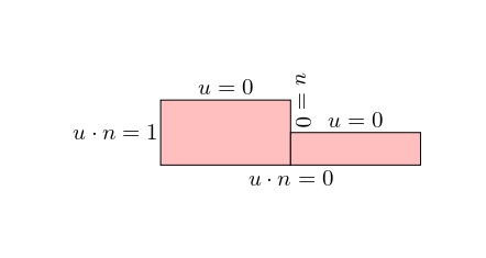
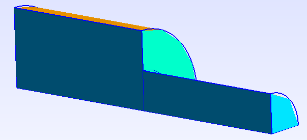
The geometry is created using GMSH. Two different pipelines are proposed. It consists in two quarter of cylinders of different heights with an inflow imposed on the left side and a no slip condition for the upper sides.
The objective is to find the resulting velocity and pressure.
Implementation#
Given the strong compatibility between GMSH and FEniCSx it is recommended to use GMSH. GMSH also has a python API. The mesh, refinement and marking operations can be proceeded in GMSH and imported in the FEniCSx environment.
Geomerty creation using GMSH#
From a 2D Geometry#
For this example we start from the 2D geometry generated for the 2D Stoke example and we apply a revolution operation. Similarly, an extrusion operation can be operated within GMSH.
Libraries and settings#
As for any GMSH API code, one must first import the libraries
import gmsh
import numpy
import sys
The geometrical and dimension of the problem can then be specified:
L1 = 2.
H1 = 1.
L2 = 2.
H2 = 0.5
# Dimension of the problem,
gdim = 3
The gmsh model is initialised with its internal settings specified:
gmsh.initialize()
gmsh.clear()
gmsh.model.add("3D_Stokes")
#Characteristic length
lc = (L1+L2)/50
gmsh.model.occ.synchronize()
gmsh.option.setNumber("General.Terminal",1)
gmsh.option.setNumber("Mesh.Optimize", True)
gmsh.option.setNumber("Mesh.OptimizeNetgen", True)
gmsh.option.setNumber("Mesh.MeshSizeMin", 0.1*lc)
gmsh.option.setNumber("Mesh.MeshSizeMax", lc)
gmsh.model.occ.synchronize()
# gmsh.option.setNumber("Mesh.MshFileVersion", 2.0)
# gmsh.option.setNumber("Mesh.MeshSizeExtendFromBoundary", 0.002)
# gmsh.option.setNumber("Mesh.MeshSizeFromPoints", 0)
# gmsh.option.setNumber("Mesh.MeshSizeFromCurvature", 5)
Geometry#
To compute the geometry, we first generate the rectangles:
# Left square
A = [0, 0]
C = [L1, H1]
D = [L1, 0]
# Right square
E = [(L1+L2), H2]
#
# gmsh.model.occ.addRectangle(x, y, z, dx, dy, tag=-1, roundedRadius=0.)
s1 = gmsh.model.occ.addRectangle(A[0], A[1], 0, L1, H1, tag=-1)
s2 = gmsh.model.occ.addRectangle(D[0], D[1], 0, L2, H2, tag=-1)
#
gmsh.model.occ.synchronize()
Then, we operate a revolution operation:
# gmsh.model.occ.revolve(dimTags, x, y, z, ax, ay, az, angle, numElements=[], heights=[], recombine=False)
gmsh.model.occ.revolve([(2,s1),(2,s2)], 0,0,0, 1, 0, 0, -numpy.pi/2)
gmsh.model.occ.synchronize()
As a safeguard, we ensure removing all duplicates and export the geometry fot control:
gmsh.model.occ.removeAllDuplicates()
#
gmsh.model.occ.synchronize()
gmsh.write('3D_Stokes.geo_unrolled')
Marking#
GMSH creates the mesh for physical groups. Each of these groups are marked. All lines, surfaces and volumes of the model can be listed with:
lines, surfaces, volumes = [gmsh.model.getEntities(d) for d in [1, 2, 3]]
boundaries = gmsh.model.getBoundary(volumes, oriented=False)
It is then required to create empty lists and tag values:
left, top_left, middle_up, top_right, right, bottom, front = [], [], [], [], [], [], []
tag_left, tag_top_left, tag_middle_up, tag_top_right, tag_right, tag_bottom, tag_front = 1, 2, 3, 4, 5, 6,7
left_vol, right_vol = [], []
tag_left_vol, tag_right_vol = 10, 20
The lists can be automatically filled by identification of the faces and volumes based on their center of mass position:
for boundary in boundaries:
  center_of_mass = gmsh.model.occ.getCenterOfMass(boundary[0], boundary[1])
  if numpy.isclose(center_of_mass[0],0):
    left.append(boundary[1])
  elif (center_of_mass[0]>H2) and (center_of_mass[1]>H2):
    top_left.append(boundary[1])
  elif numpy.isclose(center_of_mass[0],L1):
    middle_up.append(boundary[1])
  elif numpy.isclose(center_of_mass[0],L1+L2):
    right.append(boundary[1])
  elif numpy.isclose(center_of_mass[1],0):
    bottom.append(boundary[1])
  elif numpy.isclose(center_of_mass[2],0):
    front.append(boundary[1])
  else:
    top_right.append(boundary[1])
Alternatively they can be hand filled using the geo_unrolled filed and visualizing in the GMSH GUI.
To assign the surface tags, we run the following:
gmsh.model.addPhysicalGroup(gdim-1, left, tag_left)
gmsh.model.setPhysicalName(gdim-1, tag_left, 'Left')
#
gmsh.model.addPhysicalGroup(gdim-1, top_left, tag_top_left)
gmsh.model.setPhysicalName(gdim-1, tag_top_left, 'Top_left')
#
gmsh.model.addPhysicalGroup(gdim-1, middle_up, tag_middle_up)
gmsh.model.setPhysicalName(gdim-1, tag_middle_up, 'Middle_up')
#
gmsh.model.addPhysicalGroup(gdim-1, top_right, tag_top_right)
gmsh.model.setPhysicalName(gdim-1, tag_top_right, 'Top_right')
#
gmsh.model.addPhysicalGroup(gdim-1, right, tag_right)
gmsh.model.setPhysicalName(gdim-1, tag_right, 'Right')
#
gmsh.model.addPhysicalGroup(gdim-1, bottom, tag_bottom)
gmsh.model.setPhysicalName(gdim-1, tag_bottom, 'Bottom')
#
gmsh.model.addPhysicalGroup(gdim-1, front, tag_front)
gmsh.model.setPhysicalName(gdim-1, tag_front, 'Front')
Similarly for the volumes:
for volume in volumes:
  center_of_mass = gmsh.model.occ.getCenterOfMass(volume[0], volume[1])
  if center_of_mass[0]<L1:
    left_vol.append(volume[1])
  else:
    right_vol.append(volume[1])
#
gmsh.model.addPhysicalGroup(gdim, left_vol, tag_left_vol)
gmsh.model.setPhysicalName(gdim, tag_left_vol, 'left')
#
gmsh.model.addPhysicalGroup(gdim, right_vol, tag_right_vol)
gmsh.model.setPhysicalName(gdim, tag_right_vol, 'right')
Once again it is recommended to check the geometry identification:
gmsh.model.occ.synchronize()
gmsh.write('3D_Stokes_marked.geo_unrolled')
The mesh is generated and exported:
gmsh.model.mesh.generate(gdim)
gmsh.write("3D_Stokes_mesh.msh")
Executing the following command at the end run the GMSH Gui for visualization before finalizing the model:
if 'close' not in sys.argv:
    gmsh.fltk.run()
gmsh.finalize()
From elementary geometries#
When you have elementary entities defining your domain, it is often easier to use them and use boolean operations (cut,fragment,fuse,etc.). In the present case the Geometry could be created simply with two cylinders.
The beginning is the same:
#----------------------------------------------------------------------
# Libraries
#----------------------------------------------------------------------
#
import gmsh
import numpy
import sys
#
#----------------------------------------------------------------------
# Geometrical parameters
#----------------------------------------------------------------------
L1 = 2.
H1 = 1.
L2 = 2.
H2 = 0.5
# Dimension of the problem,
gdim = 3
#----------------------------------------------------------------------
#
#----------------------------------------------------------------------
# Set options
#----------------------------------------------------------------------
#
gmsh.initialize()
gmsh.clear()
gmsh.model.add("3D_Stokes")
#Characteristic length
lc = (L1+L2)/60
gmsh.model.occ.synchronize()
gmsh.option.setNumber("General.Terminal",1)
gmsh.option.setNumber("Mesh.Optimize", True)
gmsh.option.setNumber("Mesh.OptimizeNetgen", True)
gmsh.option.setNumber("Mesh.MeshSizeMin", 0.1*lc)
gmsh.option.setNumber("Mesh.MeshSizeMax", lc)
gmsh.model.occ.synchronize()
# gmsh.option.setNumber("Mesh.MshFileVersion", 2.0)
# gmsh.option.setNumber("Mesh.MeshSizeExtendFromBoundary", 0.002)
# gmsh.option.setNumber("Mesh.MeshSizeFromPoints", 0)
# gmsh.option.setNumber("Mesh.MeshSizeFromCurvature", 5)
Then, two cylinders are added and our geometry is finished:
# gmsh.model.occ.addCylinder(x, y, z, dx, dy, dz, r, tag=-1, angle=2*pi)
cylinder = gmsh.model.occ. addCylinder(0 ,0 ,0 ,L1 ,0 ,0 ,H1,tag =10 , angle=numpy.pi/2)
gmsh.model.occ. synchronize ()
cylinder2 = gmsh.model.occ. addCylinder(L1 ,0 ,0 ,L2 ,0 ,0 ,H2,tag =20 , angle=numpy.pi/2)
gmsh.model.occ. synchronize ()
The duplicates are removed and a check file is generated.
# Remove duplicate entities and synchronize
gmsh.model.occ.removeAllDuplicates()
#
gmsh.model.occ.synchronize()
gmsh.write('3D_Stokes.geo_unrolled')
All the following steps (marking, meshing) are the same as previously:
#----------------------------------------------------------------------
# Create physical group for mesh generation and tagging
#----------------------------------------------------------------------
#
lines, surfaces, volumes = [gmsh.model.getEntities(d) for d in [1, 2, 3]]
boundaries = gmsh.model.getBoundary(volumes, oriented=False)
#
left, top_left, middle_up, top_right, right, bottom, front = [], [], [], [], [], [], []
tag_left, tag_top_left, tag_middle_up, tag_top_right, tag_right, tag_bottom, tag_front = 1, 2, 3, 4, 5, 6,7
left_vol, right_vol = [], []
tag_left_vol, tag_right_vol = 10, 20
#
for boundary in boundaries:
  center_of_mass = gmsh.model.occ.getCenterOfMass(boundary[0], boundary[1])
  if numpy.isclose(center_of_mass[0],0):
    left.append(boundary[1])
  elif (center_of_mass[0]>H2) and (center_of_mass[1]<-H2):
    top_left.append(boundary[1])
  elif numpy.isclose(center_of_mass[0],L1):
    middle_up.append(boundary[1])
  elif numpy.isclose(center_of_mass[0],L1+L2):
    right.append(boundary[1])
  elif numpy.isclose(center_of_mass[1],0):
    bottom.append(boundary[1])
  elif numpy.isclose(center_of_mass[2],0):
    front.append(boundary[1])
  else:
    top_right.append(boundary[1])
#
gmsh.model.addPhysicalGroup(gdim-1, left, tag_left)
gmsh.model.setPhysicalName(gdim-1, tag_left, 'Left')
#
gmsh.model.addPhysicalGroup(gdim-1, top_left, tag_top_left)
gmsh.model.setPhysicalName(gdim-1, tag_top_left, 'Top_left')
#
gmsh.model.addPhysicalGroup(gdim-1, middle_up, tag_middle_up)
gmsh.model.setPhysicalName(gdim-1, tag_middle_up, 'Middle_up')
#
gmsh.model.addPhysicalGroup(gdim-1, top_right, tag_top_right)
gmsh.model.setPhysicalName(gdim-1, tag_top_right, 'Top_right')
#
gmsh.model.addPhysicalGroup(gdim-1, right, tag_right)
gmsh.model.setPhysicalName(gdim-1, tag_right, 'Right')
#
gmsh.model.addPhysicalGroup(gdim-1, bottom, tag_bottom)
gmsh.model.setPhysicalName(gdim-1, tag_bottom, 'Bottom')
#
gmsh.model.addPhysicalGroup(gdim-1, front, tag_front)
gmsh.model.setPhysicalName(gdim-1, tag_front, 'Front')
#
for volume in volumes:
  center_of_mass = gmsh.model.occ.getCenterOfMass(volume[0], volume[1])
  if center_of_mass[0]<L1:
    left_vol.append(volume[1])
  else:
    right_vol.append(volume[1])
#
print(surfaces)
gmsh.model.addPhysicalGroup(gdim, left_vol, tag_left_vol)
gmsh.model.setPhysicalName(gdim, tag_left_vol, 'left')
#
gmsh.model.addPhysicalGroup(gdim, right_vol, tag_right_vol)
gmsh.model.setPhysicalName(gdim, tag_right_vol, 'right')
#
gmsh.model.occ.synchronize()
gmsh.write('3D_Stokes_marked.geo_unrolled')
#
gmsh.model.mesh.generate(gdim)
gmsh.write("3D_Stokes_mesh.msh")
if 'close' not in sys.argv:
    gmsh.fltk.run()
gmsh.finalize()
Finite Element Computation#
Libraries#
Computing the Finite element problem within FEniCSx in python requires to load the libraries:
import dolfinx
import ufl
import basix
import mpi4py
import petsc4py
from dolfinx.fem.petsc import NonlinearProblem
from dolfinx.nls.petsc import NewtonSolver
One can assess the version of FEniCSx with the following:
print("Dolfinx version is:",dolfinx.__version__)
Mesh Loading#
We load the mesh, facet and cell tags from the msh file created:
mesh, cell_tag, facet_tag = dolfinx.io.gmshio.read_from_msh('./3D_Stokes_mesh.msh', mpi4py.MPI.COMM_WORLD, 0, gdim=3)
Function spaces, Functions and expressions#
For stability reasons, we create a mixed element P2vxP1 for (u,p) to solve the Stokes problem:
# Finite Element
P1       = basix.ufl.element("P", mesh.topology.cell_name(), degree=1)
# Vector Element
P1_v     = basix.ufl.element("P", mesh.topology.cell_name(), degree=1, shape=(mesh.topology.dim,))
P2_v     = basix.ufl.element("P", mesh.topology.cell_name(), degree=2, shape=(mesh.topology.dim,))
# Mixed element
MxE      = basix.ufl.mixed_element([P1,P2_v])
The associated function spaces with the element types are:
P1v_space = dolfinx.fem.functionspace(mesh, P1_v)
CHS       = dolfinx.fem.functionspace(mesh, MxE)
tensor_space = dolfinx.fem.functionspace(mesh, tensor_elem)
One can then specify the functions and if needed their expression for interpolation:
u_export      = dolfinx.fem.Function(P1v_space)
u_export.name = "u"
#
sol    = dolfinx.fem.Function(CHS)
q, w   = ufl.TestFunctions(CHS)
# Solution vector
p, u   = ufl.split(sol)
#
# Definition of the normal vector
n      = ufl.FacetNormal(mesh)
The operators are also defined at this point:
# Specify the desired quadrature degree
q_deg = 4
# Redefinition dx and ds
dx    = ufl.Measure('dx', metadata={"quadrature_degree":q_deg}, subdomain_data=cell_tag, domain=mesh)
ds    = ufl.Measure("ds", domain=mesh, subdomain_data=facet_tag)
Boundary conditions#
Three different type of dirichlet boundary conditions are introduced:
no-slip conditions for the velocity on the top left / top right and top middle boundaries,
inflow of v_x=1 on the left boundary,
Symmetry condition v_y=0 on the bottom boundary,
Symmetry condition v_z=0 on the front boundary.
bcs = []
fdim = mesh.topology.dim - 1
#
def add_dirichlet_BC(functionspace,dimension,facet,value):
  dofs   = dolfinx.fem.locate_dofs_topological(functionspace, dimension, facet)
  bcs.append(dolfinx.fem.dirichletbc(value, dofs, functionspace))
#
# No-slip boundary condition for velocity
# top left
add_dirichlet_BC(CHS.sub(1).sub(0),fdim,facet_tag.find(2), petsc4py.PETSc.ScalarType(0.))
add_dirichlet_BC(CHS.sub(1).sub(1),fdim,facet_tag.find(2), petsc4py.PETSc.ScalarType(0.))
add_dirichlet_BC(CHS.sub(1).sub(2),fdim,facet_tag.find(2), petsc4py.PETSc.ScalarType(0.))
# top right
add_dirichlet_BC(CHS.sub(1).sub(0),fdim,facet_tag.find(4), petsc4py.PETSc.ScalarType(0.))
add_dirichlet_BC(CHS.sub(1).sub(1),fdim,facet_tag.find(4), petsc4py.PETSc.ScalarType(0.))
add_dirichlet_BC(CHS.sub(1).sub(2),fdim,facet_tag.find(4), petsc4py.PETSc.ScalarType(0.))
# middle up
add_dirichlet_BC(CHS.sub(1).sub(0),fdim,facet_tag.find(3), petsc4py.PETSc.ScalarType(0.))
add_dirichlet_BC(CHS.sub(1).sub(1),fdim,facet_tag.find(3), petsc4py.PETSc.ScalarType(0.))
add_dirichlet_BC(CHS.sub(1).sub(2),fdim,facet_tag.find(3), petsc4py.PETSc.ScalarType(0.))
#
# inflow vx = 1 left side
add_dirichlet_BC(CHS.sub(1).sub(0),fdim,facet_tag.find(1), petsc4py.PETSc.ScalarType(1.))
add_dirichlet_BC(CHS.sub(1).sub(1),fdim,facet_tag.find(1), petsc4py.PETSc.ScalarType(0.))
add_dirichlet_BC(CHS.sub(1).sub(2),fdim,facet_tag.find(1), petsc4py.PETSc.ScalarType(0.))
#
# Symmetry plan vy = 0 bottom
add_dirichlet_BC(CHS.sub(1).sub(1),fdim,facet_tag.find(6), petsc4py.PETSc.ScalarType(0.))
#
# Symmetry plan vz = 0 front
add_dirichlet_BC(CHS.sub(1).sub(2),fdim,facet_tag.find(7), petsc4py.PETSc.ScalarType(0.))
Variational form#
The objective is to find (u,p), such that we have the following variationnal form:
This can be introduced as:
b = dolfinx.fem.Constant(mesh,(0.0, 0.0, 0.0))
F = ufl.inner(ufl.grad(u), ufl.grad(w))*dx + ufl.div(w)*p*dx + q*ufl.div(u)*dx - ufl.inner(b, w)*dx
Solving and Post-Processing#
To have the full computation log, the following is required. These information are crucial when debugging.
#----------------------------------------------------------------------
# Debug instance
log_solve=True
if log_solve:
    from dolfinx import log
    log.set_log_level(log.LogLevel.INFO)
#----------------------------------------------------------------------
We solve the problem using the nonlinear approach:
problem = NonlinearProblem(F, sol, bcs)
solver = NewtonSolver(mesh.comm, problem)
#
# Absolute tolerance
solver.atol                  = 1e-8
# relative tolerance
solver.rtol                  = 1e-8
# Convergence criterion
solver.convergence_criterion = "incremental"
# Maximum iterations
solver.max_it                = 15
# Solver Pre-requisites
ksp                                               = solver.krylov_solver
opts                                              = petsc4py.PETSc.Options()
option_prefix                                     = ksp.getOptionsPrefix()
opts[f"{option_prefix}ksp_type"]                  = "preonly"
opts[f"{option_prefix}pc_type"]                   = "lu"
opts[f"{option_prefix}pc_factor_mat_solver_type"] = "mumps"
ksp.setFromOptions()
num_its, converged = solver.solve(sol)
sol.x.scatter_forward()
Once the problem is solved, we can apply the post processing:
# Get sub-functions
p_, u_ = sol.split()
p_.name = "p"
#
u_expr = dolfinx.fem.Expression(sol.sub(1),P1v_space.element.interpolation_points())
u_export.interpolate(u_expr)
u_export.x.scatter_forward()
At this point the quantities are saved in an xdmf file:
xdmf = dolfinx.io.XDMFFile(mesh.comm, "3D_Stokes.xdmf", "w")
xdmf.write_mesh(mesh)
t=0
xdmf.write_function(u_export,t)
xdmf.write_function(p_,t)
xdmf.write_function(strainrate,t)
xdmf.write_function(stress,t)
One can further represent the velocity field with glyphs using pyvista:
import pyvista
import numpy
pyvista.start_xvfb()
topology, cell_types, geometry = dolfinx.plot.vtk_mesh(P1v_space)
values = numpy.zeros((geometry.shape[0], 3), dtype=numpy.float64)
values[:, :len(u_export)] = u_export.x.array.real.reshape((geometry.shape[0], len(u_export)))

# Create a point cloud of glyphs
function_grid = pyvista.UnstructuredGrid(topology, cell_types, geometry)
function_grid["u"] = values
glyphs = function_grid.glyph(orient="u", factor=0.1)

# Create a pyvista-grid for the mesh
grid = pyvista.UnstructuredGrid(*dolfinx.plot.vtk_mesh(mesh, mesh.topology.dim))

# Create plotter
plotter = pyvista.Plotter()
# plotter.add_mesh(grid, style="wireframe", color="k")
plotter.add_mesh(grid, color="grey", ambient=0.02, opacity=0.05 , show_edges=False)
plotter.add_mesh(glyphs, cmap='coolwarm')
plotter.update_scalar_bar_range([1, 8])
plotter.view_vector((0, 3, -20))
plotter.show_axes()
# plotter.view_xy()
plotter.save_graphic('Result.pdf')
plotter.close()